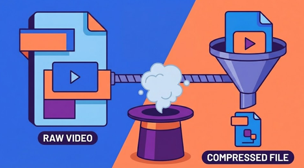
The Art of Compression - How Codecs Cheat Physics

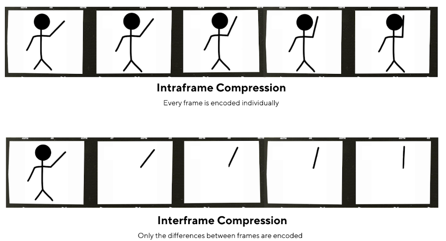
1 Spatial Compression (Intra-frame): How an I-Frame Compresses a Single Picture

In video compression, an I-frame (Intra-frame or Keyframe) is a frame that is compressed independently, without relying on information from past or future frames. Conceptually, it behaves much like a JPEG image inside a video stream. Understanding how an I-frame works is essential because it forms the foundation upon which more advanced temporal compression techniques are built.

This section explains how a single image is reduced in size through spatial compression while preserving visual quality.

What Is Spatial Compression?

Spatial compression focuses on reducing redundancy within a single frame. A raw image contains millions of pixels, but many of those pixels are visually similar. Instead of storing every pixel exactly as captured, modern codecs store mathematical descriptions of patterns and structures.

The goal is simple: represent the same visual information using fewer bits by exploiting how images are structured and how humans perceive detail.

Step 1: Dividing the Frame into Blocks

The first stage of intra-frame compression involves splitting the image into small square regions, often called blocks or macroblocks. Common sizes include 16×16 or 8×8 pixels.

This block-based approach works because nearby pixels tend to share similar colors and textures. A blue sky, a wall, or a blurred background contains large regions with minimal variation. By analyzing small sections independently, the encoder can identify patterns more efficiently.

Breaking the image into blocks also allows localized compression. Highly detailed areas can retain more information, while smooth regions can be compressed aggressively.

Step 2: Transforming Pixels into Frequencies (Discrete Cosine Transform)

Once the frame is divided into blocks, each block undergoes a mathematical operation known as the Discrete Cosine Transform (DCT).

Instead of representing an image as raw pixel values, the DCT converts spatial information into frequency components:

• Low frequencies describe broad shapes and smooth color transitions.
• High frequencies represent fine textures, edges, and noise.

This transformation is crucial because human vision is far more sensitive to low-frequency information than to extremely fine detail. By working in the frequency domain, the encoder gains the ability to selectively reduce less important data without significantly affecting perceived quality.

Step 3: Quantization - The Core of Compression

Quantization is where most of the file size reduction happens.

After the frequency transform, the encoder reduces precision in the high-frequency components. Small variations and subtle details are rounded or removed, which decreases the amount of information that must be stored.

For example, a precise value might be rounded to a simpler approximation. While this introduces a small loss of detail, the change is usually imperceptible to viewers.

Quantization is also responsible for familiar compression artifacts. When compression becomes aggressive, edges may appear blocky or fine textures may look smeared. These effects arise because the encoder has discarded too much high-frequency information.

In essence, quantization trades mathematical accuracy for visual efficiency.

Step 4: Entropy Encoding - Storing Data Efficiently

After quantization, the remaining data is encoded using entropy coding techniques such as run-length encoding, Huffman coding, or context-adaptive binary arithmetic coding (CABAC).

At this stage, the encoder does not change visual quality; instead, it reduces redundancy in how data is written to the file. Repeated values and predictable patterns are stored using shorter representations, further shrinking the final size of the I-frame.

Why I-Frames Exist in Video Codecs

Although I-frames are larger than other frame types, they serve a critical purpose. Because they are self-contained, they allow video players to:

• Seek to different timestamps quickly.
• Recover from transmission errors.
• Provide reference points for inter-frame compression.

Between I-frames, codecs typically store only the differences between frames, resulting in significantly smaller file sizes. However, without periodic I-frames, decoding would become unstable and navigation would be difficult.

Conceptual Model

The process of intra-frame compression can be summarized as a pipeline:

1. Split the frame into blocks.
2. Transform each block into frequency data using DCT.
3. Apply quantization to remove visually insignificant detail.
4. Encode the remaining information efficiently.

Rather than storing millions of independent pixels, the encoder stores a structured description of patterns and variations. This is why compression feels like “cheating physics”: the visual result appears nearly identical, yet the data required to represent it is dramatically smaller.

2 Temporal Compression (Inter-frame): Motion Vectors, P-Frames, and

B-Frames

While intra-frame compression reduces redundancy inside a single image, the real efficiency of modern video codecs comes from temporal compression, also called inter-frame compression. Instead of treating every frame as a completely new picture, the encoder analyzes how pixels move over time and stores only the changes between frames.

This approach dramatically reduces file size because most video scenes contain large areas that remain similar from one frame to the next. Rather than saving repeated visual information, the codec records mathematical descriptions of motion and difference.

The Core Idea: Frames Are Often Similar

Consider a person walking across a static background. From one frame to the next:

• The background barely changes.
• Only a small region moves.
• Many pixels simply shift position.

If each frame were stored independently, the same background would be encoded repeatedly. Temporal compression avoids this redundancy by predicting new frames based on previously decoded ones.

This is where motion estimation and motion vectors come into play.

Motion Vectors: Describing Movement Instead of Storing Pixels

A motion vector is a small piece of data that describes how a block of pixels has moved between frames.

During encoding, the video is again divided into blocks. The encoder searches previous or future frames to find where a similar block exists. If a match is found, instead of storing the block again, the codec records:

• The position of the reference block.
• The direction and distance it moved.

For example, if an object shifts slightly to the right, the encoder can write instructions such as:

“Take this block from the previous frame and move it 4 pixels to the right.”

This transforms video into a sequence of instructions about motion, rather than a sequence of independent images.

P-Frames (Predictive Frames)

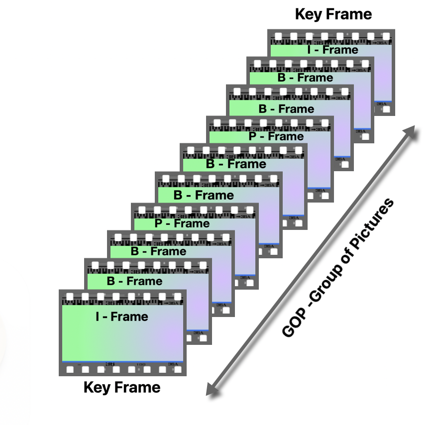
A P-frame predicts its content using information from a previous reference frame, usually an I-frame or another P-frame.

Instead of storing the entire image, a P-frame contains:

• Motion vectors that describe how blocks have moved.
• Residual data that captures any differences the motion prediction could not reproduce.

In practical terms, a P-frame answers the question:

“How does this frame differ from the last one?”

Because only motion and changes are stored, P-frames are significantly smaller than I-frames.

However, P-frames depend on earlier frames for decoding. If a reference frame is missing or corrupted, subsequent P-frames may also be affected because the prediction chain breaks.

B-Frames (Bi-directional Frames)

A B-frame extends the idea of prediction by referencing both past and future frames. Instead of predicting solely from what came before, the encoder analyzes motion across multiple directions in time.

This allows the codec to choose the most efficient prediction:

• Forward prediction from earlier frames.
• Backward prediction from later frames.
• Or an interpolation between both.

Because B-frames have access to more contextual information, they often achieve higher compression efficiency than P-frames. They represent the frame as a blend of motion and differences derived from surrounding frames.

Conceptually, a B-frame answers:

“Given what happened before and after, what is the most efficient way to reconstruct this frame?”

Why Video Becomes “Math Instructions”

When temporal compression is applied, the video file stops being a simple collection of pictures. Instead, it becomes a structured set of instructions:

• Reference this earlier frame.
• Shift these blocks using motion vectors.
• Apply small corrections where predictions are imperfect.

In many scenes, especially those with slow camera movement or static backgrounds, large portions of frames can be reconstructed using only motion data. The actual pixel data stored in the file becomes minimal compared to raw video.

This is why modern codecs achieve dramatic compression ratios. Rather than storing every pixel repeatedly, they store how pixels evolve over time.

Residual Data: Correcting Prediction Errors

Motion prediction is rarely perfect. Lighting changes, occlusions, and complex motion introduce differences between predicted and actual frames.

To handle this, the encoder stores a residual - the remaining difference after motion compensation. Residuals are typically compressed using the same spatial techniques described in intra-frame compression, including transforms and quantization.

The final decoded frame is reconstructed by combining:

• The predicted motion-based frame.
• The residual correction data.

Trade-offs and Compression Structure

A typical video stream alternates between I-frames, P-frames, and B-frames:

• I-frames provide independent reference points.
• P-frames reduce redundancy by predicting forward in time.
• B-frames maximize efficiency by predicting in both directions.

Increasing the number of inter-frames improves compression but also increases decoding complexity and dependency between frames. This balance is carefully tuned by the encoder depending on bitrate, latency requirements, and playback constraints.

3 Bitrate vs. Density (The BPP Metric): Understanding CBR, VBR, and Bits Per Pixel

In video compression, bitrate is often the first number people look at when judging quality. However, bitrate alone does not describe how much visual information is being preserved. Two videos can share the same bitrate yet look completely different depending on their resolution, motion complexity, and encoding strategy.

To properly understand compression efficiency, it helps to think in terms of data density - how many bits are allocated per pixel. This is where the concept of Bits Per Pixel (BPP) becomes useful, especially when building scripts or automated encoding pipelines.

Bitrate: The Flow of Data Over Time

Bitrate refers to how many bits are used to represent video per second, usually expressed in kbps or Mbps. It controls the overall size of a video file and the amount of information available for compression.

A higher bitrate allows the encoder to preserve more detail, while a lower bitrate forces the encoder to discard more information through quantization and prediction.

However, bitrate by itself is incomplete because it does not account for resolution. A 1080p video and a 4K video at the same bitrate do not receive the same amount of data per pixel. The 4K video must spread that data across far more pixels, which can reduce visual clarity.

Constant Bitrate (CBR)

Constant Bitrate (CBR) maintains a steady data rate throughout the entire video. Regardless of whether a scene is simple or complex, the encoder tries to output roughly the same number of bits every second.

Characteristics of CBR

• Predictable file size and bandwidth usage.
• Useful for live streaming or systems with strict network limits.
• Less efficient in scenes where visual complexity changes.

In a static scene, CBR may waste bits because fewer details need encoding. In a highly dynamic scene, it may struggle to maintain quality because the bitrate ceiling cannot increase to accommodate complexity.

CBR prioritizes consistency and stability rather than optimal compression efficiency.

Variable Bitrate (VBR)

Variable Bitrate (VBR) allows the encoder to adjust bitrate depending on the visual complexity of each moment.

• Complex scenes receive more bits.
• Simple scenes receive fewer bits.

This dynamic allocation usually produces better visual quality at the same average file size because the encoder distributes bits where they are most needed.

Characteristics of VBR

• More efficient compression.
• Higher quality for the same average bitrate.
• Less predictable instantaneous bandwidth.

Most offline video encoding workflows prefer VBR because it balances quality and storage more effectively than CBR.

Bits Per Pixel (BPP): Measuring Data Density

While bitrate measures data over time, Bits Per Pixel (BPP) measures how much data is assigned to each individual pixel. It provides a normalized way to compare videos of different resolutions.

A simplified conceptual formula is:

BPP ≈ Bitrate / (Width × Height × Frames Per Second)

This value represents the density of information allocated to the visual content. Higher BPP generally indicates:

• More preserved detail.
• Less aggressive compression.
• Higher visual fidelity.

Lower BPP indicates heavier compression and a greater likelihood of artifacts such as blockiness or blurring.

Why BPP Matters More Than Bitrate Alone

Consider two videos:

• Video A: 1080p at 5 Mbps
• Video B: 4K at 5 Mbps

Although both share the same bitrate, Video B has four times as many pixels. Each pixel receives fewer bits, resulting in a lower BPP. The encoder must compress more aggressively, which may reduce sharpness or introduce artifacts.

BPP provides a resolution-aware way to judge quality targets. Instead of guessing a bitrate for every resolution, encoding pipelines can calculate bitrate based on a desired BPP range.

How Encoding Scripts Use BPP

In automated encoding workflows, BPP is often used as a guiding metric for selecting a target bitrate.

Rather than hardcoding specific bitrates for every resolution, a script can:

1. Read the video’s width, height, and frame rate.
2. Choose a target BPP value based on desired quality.
3. Calculate an estimated bitrate from that BPP.

This approach makes encoding more consistent across different resolutions and content types. A 720p clip and a 4K clip can be encoded with comparable visual density even though their final bitrates differ significantly.

Your Python script likely relies on BPP because it offers a scalable way to control quality without manually tuning bitrate for each input file.

Typical BPP Ranges (Conceptual Guidelines)

Although exact values depend on codec efficiency and content type, general ranges often look like this:

• Very low quality or heavy compression: below 0.05
• Streaming-friendly compression: around 0.07–0.15
• High-quality encoding: around 0.15–0.30 or higher

Fast motion, grain, and detailed textures may require higher BPP values to maintain clarity.

4 Constant Rate Factor (CRF): Quality-Driven Encoding Instead of Fixed Bitrates

Traditional encoding methods often revolve around choosing a specific bitrate and forcing the video to fit within that constraint. While this approach is predictable, it does not always produce consistent visual quality. Modern codecs introduced Constant Rate Factor (CRF) as a more intelligent alternative - a method that targets perceived quality rather than a fixed data rate.

CRF changes the philosophy of encoding from “How big should the file be?” to “How good should the video look?”

The Problem with Fixed Bitrates

When using constant or average bitrate targets, the encoder is restricted by a predetermined amount of data per second. This creates a mismatch between bitrate and scene complexity.

• Simple scenes may receive more bits than necessary, wasting space.
• Complex scenes may not receive enough bits, leading to visible artifacts.

Because visual complexity varies throughout a video, a single bitrate cannot optimally serve every moment. The result is often inconsistent quality: some scenes look overly compressed while others use excessive bandwidth.

What Is CRF?

Constant Rate Factor is a quality-based encoding mode used in many modern encoders, such as those built around H.264 and H.265. Instead of defining how many bits the encoder must use, CRF defines a target level of compression strength.

The encoder dynamically adjusts bitrate to maintain consistent visual quality across the entire video:

• Easy-to-compress scenes use fewer bits.
• Complex scenes automatically receive more bits.

The CRF value itself represents a scale of quality versus compression. Lower CRF values preserve more detail and produce larger files, while higher values increase compression and reduce file size.

How CRF Works Internally

CRF operates by controlling the level of quantization applied during encoding. Recall that quantization determines how much detail is discarded from frequency data during compression.

Instead of applying the same quantization across all scenes, CRF allows the encoder to:

1. Analyze frame complexity.
2. Adjust quantization strength dynamically.
3. Allocate bits where visual detail requires it.

If a frame contains motion, grain, or intricate textures, the encoder lowers quantization to preserve detail. If a frame is smooth or static, quantization increases to reduce file size.

This adaptive behavior creates a balance between quality and efficiency without requiring manual bitrate tuning.

Why CRF Is Often Superior to Fixed Bitrates

1. Consistent Perceived Quality

CRF aims to maintain similar visual fidelity throughout a video. Instead of forcing every second to consume the same number of bits, it responds to what the viewer actually sees.

2. Efficient File Sizes

Because bits are only used when necessary, CRF often produces smaller files than constant bitrate encoding while maintaining equal or better quality.

3. Reduced Manual Tuning

Fixed bitrate workflows require different settings for different resolutions and content types. CRF simplifies this by letting a single quality value scale automatically across various inputs.

4. Better Handling of Complex Motion

High-motion scenes naturally require more data. CRF allows bitrate spikes when needed, avoiding the blockiness that can occur when a fixed bitrate becomes insufficient.

CRF vs. CBR vs. VBR

Although CRF and VBR both allow bitrate to change dynamically, they differ in intent:

• CBR (Constant Bitrate) focuses on stable data output, useful for streaming constraints.
• VBR (Variable Bitrate) targets an average bitrate over time.
• CRF targets visual quality and lets bitrate emerge naturally.

CRF can be thought of as a quality-first form of variable bitrate encoding. Instead of distributing bits to match a predefined average, it distributes bits to maintain a consistent visual standard.

Understanding the CRF Scale

The CRF scale varies slightly by codec, but generally:

• Lower numbers mean higher quality and larger files.
• Higher numbers mean stronger compression and smaller files.

For many workflows, values in the low-to-mid range produce visually transparent results. However, optimal values depend on content characteristics such as motion, grain, and resolution.

Importantly, CRF does not guarantee a specific file size. Two videos encoded with the same CRF value may produce very different bitrates depending on how complex the content is.

When CRF Is the Right Choice

CRF is ideal for:

• Archival-quality encoding where visual consistency matters.
• Offline processing where exact file size is not critical.
• Automated pipelines where manual bitrate selection is impractical.

However, CRF is not always suitable for scenarios requiring strict bandwidth control, such as live streaming or environments with limited network capacity.